
Mixture of Experts, Sparsity, and Megablocks


We’d like to thank Trevor Gale, lead-author of MegaBlocks, for his help with this piece.
Intro to Mixture of Experts
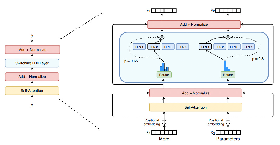
A neural network learns features that attempt to map input to output. A neural network with 3 features is almost certainly less powerful than one with 10,000 features. Features are composed by parameters and represented by neurons (albeit often in incredibly complicated and uninterpretable ways) and so increasing the number of features in a neural net generally requires increasing the parameters in our neural net. This presents the obvious problem that in order to increase the expressiveness of our neural net we need to make our neural net larger by increasing our matrices containing parameters and therefore increase our computational cost. Mixture of Experts (MoE) proposes a way to increase our network's parameter count without (in theory) increasing computation. Specifically, for every feed-forward network (FFN) in the model, we create many "versions" of it (each of which is called an expert), each with a unique set of parameters. So, instead of forcing all tokens through the same feed-forward network we send each token through the FFN "best suited” to it. See this diagram below:
We can use MoE for all sorts of data and the general principles hold so we'll stick to the NLP case for simplicity. The necessary features to optimally map a token to its correct output will naturally be different for different tokens. And so, increasing the number of experts and therefore the total number of features our network can represent should allow us to include more of the necessary features to map all tokens we see to their correct outputs. Take a standard "dense" network (meaning one FFN that every token is mapped to). So long as this FFN isn't perfect, meaning it can't map every single token to its correct output (true of every neural network to ever exist so far) or it can't map every single token to its output better than any other network of its size, there must be at least one token for which we could better map it to its output if fed through some different FFN with different parameters and presumably more suitable features. Now we add in a second FFN and opt to only send tokens through a single expert maintaining our theoretical computational cost from before (in practice, this is the big challenge with MoE and motivates MegaBlocks). This expert should increase the model's performance, because so long as it learns features such that there is one token better mapped to its output when fed through this second expert (and we only route tokens to this expert that are better mapped to output by the expert), we will achieve better performance than with our dense, single expert.
This is the idea of MoE. Put one way, increase the model's parameters (improving model performance as more parameters = more features = lower loss) without increasing computational cost. But this sort of ignores the sparsity of these parameters. I think it's better to frame MoE as enabling the model to improve its percentage of theoretically optimal features each token sees (and so features the model can use) when being mapped to an output. Note that the crucial aspect of MoE is that we can do the FFN computation in parallel (run multiple experts simultaneously) when performing batch computation.
In an MoE transformer, like Mistral’s 8x7B MoE model, the standard feed-forward layer, where each token is fed through the same FFN is simply replaced by a series of experts (8 in Mistral’s Mixtral model) and a router that sends tokens to specific experts. The number of experts a token can get sent to is a hyperparameter—1, 2, and 4 are all quite common (Mistral trained their model using 2 expert’s per token).
So the main idea thus far has been around conditional computation when it comes to experts in MoE. But how do we select which expert/experts we send each token to? MoE introduces a gating mechanism to do this. Specifically, we have a router weight matrix which transforms each token vector into logits with dimension equivalent to the number of experts; for a sequence with N tokens this looks like (N, d_embed) @ (d_embed, num experts) = (N, num experts). We then feed this vector for each token into a softmax which returns the probability of assigning the token to each of the experts—we select the top K largest probabilities where K is our hyperparameter determining number of experts per token (going forward we consider the K=1 case—each token is sent to a single expert—as it makes the rest of the piece simpler). We then permute the token matrix, meaning we group tokens assigned to the same expert together. This lets us split the token matrix into N contiguous chunks where each chunk represents the tokens assigned to expert N.

If you train an MoE you often notice that tokens are all routed to one/a few experts and some experts are entirely ignored. This is just a waste of experts; we want to make sure all our experts are involved so they each learn valuable features and every expert has certain tokens best suited to it—otherwise we are just wasting parameters. To do this, we use a load-balancing loss where our loss is minimized if each expert is sent 1/N tokens (where N is the number of experts)—the expert’s are all used equally. The formula is basically a dot product between a vector f and a vector P where each index i in f is the percent of tokens sent to expert i and each index i in P is the average probability the router assigned to tokens being sent to expert i. To minimize this loss we want the elements of f and P to be as small as possible—yes, 0 tokens assigned to expert 1 * 0 avg. probability for tokens being assigned to expert 1 contributes nothing to loss. But since small values for one expert mean large values for another expert we see that loss is minimized when all elements of f and P have value 1/N. We add this auxiliary loss to our normal cross-entropy loss and use a hyperparameter to scale how much weight is given to the auxiliary loss relative to CE loss (Fedus et al., 2022 find 10^-2 to be optimal).
One drawback of MoEs is that because each expert added to an MoE layer increases our parameter count, these models are fairly memory intensive compared to a dense counterpart with only one expert. While a dense model might fit on a single chip, an MoE version with multiple experts and, therefore, increased parameter count often will not. This presents challenges in terms of parallelizing training over multiple GPUs. MoEs also face challenges in fine-tuning, where they tend to overfit and struggle with generalization.
Challenges of MoE
Now, we’ll motivate the key issue that arises with the basic MoE architecture where tokens are simply routed to the experts they most "prefer" (as determined by the gating mechanism).
TPUs use the XLA compiler which requires all tensor shapes to be fixed and known ahead of run-time. Meanwhile, on GPUs, while there’s no compiler requirement for static tensors, we still want equally sized tensors. In order to maximize speed we want to compute our MoE layer (on GPU or TPU) in parallel which means computing the output of every expert's FFN in parallel. Every expert's FFN is a matrix multiply between the expert's weights and the group of tokens sent to the expert. The way to compute this in parallel is to use a batched matrix multiply where we batch each expert's matrix multiply together. The only issue is that in order to do this we need every matrix multiply in the batch to have the same shape, and therefore the matrix of tokens sent to each expert needs to be the same shape. Since the process of sending tokens to experts is dynamic, and we have no guarantee that the gating mechanism will send the same number of tokens to each expert, we must constrain the number of tokens sent to each expert to fit some size. On GPUs, then, we don’t need our matrices to be static but we need them to be the same size. This is very annoying.
Imagine we have 4 experts and a sequence of 100 tokens. Say our gating mechanism determines that most tokens (70/100) in the sequence are best suited to expert 1. We want to be able to send those tokens to expert 1 with the remaining 30 being distributed equally among the 3 other experts. The problem, of course, is our token matrices for each expert need to be the same size. We could fix every expert's input tensor to have a capacity of 70 tokens, which would mean, we have tons of padding in experts 2-4 in this case, all tokens are routed to their preferred expert but then obviously, if the next sequence sends 71 tokens to some expert we're out of luck.
We, therefore, really only have two choices. First, we could just specify every expert's input tensor have a capacity of 100 tokens (i.e. sequence length tokens) meaning there is no scenario in which the router sends more tokens to the expert than it has capacity for, and when it inevitably sends less than 100 (often way way less—the expectation is 25 in this case) we just zero out the rows of tokens that weren't sent and no issue... except we've basically just rendered the idea of experts useless. The whole point is to use sparsity to save computation (well really to increase our parameter/feature to computation ratio). If we have every expert pretend like it gets the full sequence this is just a dense feed-forward layer and with 4 experts we just add 4 dense layers in parallel and 4x computation for 4x params—our ratio is unchanged from the dense regime. But if we zero out the rows of tokens that aren't actually sent can't we ignore those zeros in our computation and therefore compute a matrix-multiply where we skip over the zeros, preventing any slowdown? This is the idea of sparsity and is really the core idea of MegaBlocks—we'll discuss this soon.
The other option is, instead of setting the capacity of every expert to the sequence length, essentially giving it unlimited capacity, Lekihin et al., 2021 and Fedus et al., 2022 introduce/use the idea of a capacity factor where we constrain each expert’s capacity to some value less than the total sequence length. If the router sends more tokens to the expert than the expert’s capacity factor allows for, those tokens are simply dropped—not sent to the expert. For a capacity factor x, each expert’s capacity is (# of tokens/experts)*capacity factor. Our capacity factor must always be at least 1. With 100 tokens and 4 experts, the smallest we can make the input tensor is (25, d_embed), otherwise we have <= 24 tokens in one expert so will need >=26 in another to compensate. But a capacity factor of 1 is too low. What if we have an expert that specializes in physics and our sentence is from a physics paper. Surely we want to route more than 25 tokens to that expert. And so we need to increase our capacity factor. We mentioned a scenario where a capacity of 70 tokens was needed; 70 (which would require a capacity factor of ~2.9) would surely be a more optimal capacity than 25, even if it still isn’t perfect and fails when met with routing of 71 or more. The problem is since every expert’s token matrix needs to be the same size the more we scale, the larger our matrices are (with the increased matrix size made up of padding) and the more compute we require. All we’re doing by increasing our capacity factor is getting us closer and closer to the unlimited capacity scenario (where capacity factor = number of experts) which we mentioned was computationally inefficient because it’s spent on padding. This illustrates a drawback of the dropless MoE method by Hwang et al., 2022. They attempt to use dynamic capacity factor selection where the capacity factor is the smallest number that still allows all tokens to be routed to their preferred expert. But we see that in our example with 70 tokens routed to expert 1, we have to pad experts 2-4 with lots of empty rows. When we have load-imbalanced routing, a dynamically selected capacity factor results in significant wasted computation (much the same way having no capacity factor would). So in practice we mostly scale to 1.15 or 1.25 (in our case constraining the expert’s to a capacity of 29 or 31).
This is clearly suboptimal. Ideally, we’d like to give every expert a capacity equal to sequence length—the token matrix sent to each expert is of shape (100, d_embed)—and simply skip over the tokens not sent to the expert (represented as zeros) in our matrix multiply. To figure out how we could do this, and why simply setting non-present tokens to zero and computing as normal isn’t sufficient, we must discuss sparsity.
Sparsity
Sparsity on GPUs is by default quite inefficient. There are basically three types of sparsity levels—unstructured sparsity, fine-grained structured sparsity, and coarse-grained sparsity. If you take a 100 by 100 matrix, zero out half the elements at random and attempt to compute this as a sparse matrix multiply where zeros are ignored (instead of just doing dense computation in O(100^3)), you are in the unstructured sparsity regime and will be slowed down massively. You'd need at least 95% sparsity (95% of the elements in the matrix are zero) to see performance on par with just taking your sparse matrix and computing it as a dense matrix multiply. Of course, in theory, we should expect much better performance—you can just skip the zero values in the matrix and save on computation. The problem is that unstructured sparsity is incredibly hard to exploit because the location of zeros (and therefore the location of non-sparse elements—the only values to be used in computation) is completely random. A major problem is that avoiding the zeros and only accessing the non-sparse elements from memory results in irregular memory access and more cache misses, not maximizing memory bandwidth which prefers large contiguous blocks of memory to be accessed at once (which requires the non-zero values be contiguous and not have zeros randomly interspersed). There’s also some overhead with indices required to denote which elements of the array were sparse so we can ignore those elements and still remember how to structure our output after only computing with the non-sparse values.
The second general class of sparsity is fine-grained structured sparsity. Here, instead of elements of the matrix being zero at random, there is some structure to the zeros, and this structure enables us to better exploit the sparsity for computation gains. This structure lets us reduce the irregularity of memory accesses and get some speedup over the unstructured case (how much speedup depends on the amount of sparsity and the type of structure). We are still limited, however, by the inability to do big contiguous memory accesses since our unit of sparsity is fine-grained—a single element—and so instead of having a huge patch of non-sparse or sparse elements we likely have some structure where some elements in the patch are sparse and some aren’t; this, then, prevents a big contiguous memory access of only non-sparse elements for this patch. An MoE implementation could exploit this fine-grained sparsity—give every expert a matrix equivalent to all the tokens (i.e. no capacity factor) and then if token 100 is not sent to expert 1, just zero out the elements of row 100 of expert 1’s token matrix. But, zeroing out every element of the row, is equivalent to treating the entire row as a coarser-structure and zeroing out the row itself. This brings us to coarse-grained structured sparsity.
Here, we make coarse-grained structures like blocks, sparse. This results in dramatic speedups because the sparsity is now structured in large scale contiguous structures meaning the costs associated with sparsity like irregular memory accesses resulting in lots of cache hits and generally poor bandwidth utilization are no longer particularly pressing issues. Unsurprisingly then, this is a gradient, and as the “coarseness” of the sparse-structures increase, performance relative to equivalent dense counterparts improve. With block-size of 32, block-sparse matrix multiplies outperform their dense counterparts at just 50% density, and unlike fine-grained sparsity continue to improve as sparsity increases.

MegaBlocks
MegaBlocks provides a solution to the seemingly necessary tradeoff between capacity factor and compute efficiency; get rid of the capacity factor (so essentially give every expert a capacity = sequence length), and handle non-present tokens by zeroing out a coarse-structure as opposed to individual elements of the non-present tokens. That is, move our MoE sparsity from fine-grained to coarse-grained.
Let’s consider the case with 3 experts and 100 tokens in our sequence. What we want to do is, for each expert select our x tokens, which collectively form a matrix with shape (x, d_embed) and compute the matrix multiply with the expert’s FFN weight matrix of shape (d_embed, hidden_layer). So we have (x, d_embed) @ (d_embed, hidden_layer). The standard batched matrix multiply approach (with 3 experts in our case), computes 3 of these in parallel, with x—the number of tokens sent to each expert required to be the same for each of the 3 experts. Without a capacity factor, then, we compute 3 of these (100, d_embed) @ (d_embed, hidden_layer) in parallel and simply zero out elements of each (100, d_embed) that weren’t set to that expert. That’s 200 rows of padding and only 100 rows of actual tokens. With a capacity factor, it’s more like 3 of (33, d_embed) @ (d_embed, hidden_layer) in parallel.

MegaBlocks explains that we can instead view an MoE layer as a a block diagonal matrix multiply involving two dense matrices—one containing all our tokens with shape (100, d_embed) and the other containing all our experts with shape (d_embed, 3*hidden_layer). If we compute this matrix multiply and do nothing else, this would just be equivalent to sending all 100 tokens to every expert—no routing whatsoever. Instead, we need to signal what elements of the output matrix of shape (100, 3*hidden_layer) will be sparse, based on what tokens are supposed to be sent to what experts. We call this operation a sparse-dense-dense (SDD) matrix multiply since our output is sparse and the two inputs are dense. We permute our token matrix such that the first x tokens of 100 represent those we want to send to expert 1, the next 100-x tokens represent what we want to send to expert 2 and so on. We see that the non-sparse output looks like 3 blocks along the diagonal. The output of the first x tokens and expert 1 in the top-left, the next 100-x tokens and expert 2 in the middle and the final y tokens and expert 3 in the bottom-right. Each of these 3 blocks has width/columns representing the hidden layer size of each expert and height/rows representing the number of tokens sent to the expert. With a capacity factor the non-sparse blocks are the same size because the number of tokens sent to each expert are equivalent. But in order to compute an MoE layer without a capacity factor, we want our blocks to be able to have variable sized rows. The problem is that for a block-sparse matrix multiply we need some fundamental fixed size block.
So, what MegaBlocks proposes is to use much smaller fixed-sized blocks which combine to make up variably sized larger blocks; these larger blocks represent the output of an expert and the tokens routed to it in our SDD block diagonal matrix. Imagine the output matrix for an SDD computation with 100 tokens and 3 experts with a hidden-layer size of 100 each; we have a 100x300 matrix where each each element can be viewed as a 1x1 fixed-sized blocks representing the output of a single token and a single element of the hidden_layer—(1, d_embed) @ (d_embed, 1) = (1,1). Making one of these little blocks sparse is equivalent to saying a token wasn’t sent to some expert (or really, the specific hidden unit of the expert). For the first 100 columns of the output matrix, if we make only the first 20 rows of those columns non-sparse that’s equivalent to saying the first expert was sent tokens 1-20 (from our permuted token matrix). With our 1x1 blocks we simply set blocks at positions (1,1) to (20,100) to be present and blocks (21,1) to (100,100) to be sparse. For expert 2, represented by columns 101-200 we set rows 1-20 to be sparse (since k=1 and they were already sent to expert 1) but we could set rows 21-80 to be non-sparse since this just requires setting the 1x1 blocks that correspond to those rows and columns to be present. We see that by toggling whether these smaller blocks are sparse or not we can alter the size of our larger blocks (expert output), meaning we alter the number of tokens sent to the expert. The key is that while we need some fixed block size, if we make this fixed block size smaller than the blocks representing our expert output we can, by toggling the sparsity of these smaller blocks, construct the larger expert output blocks to have different sizes.
1x1 blocks give us maximum flexibility but for the same reasons coarse-grained structured sparsity is more efficient than fine-grained, generally within the coarse-grained regime, the larger (coarser) the block the more efficient. We need to strike a balance, then, with our block size. We don’t want inflexible large blocks that are a huge fraction of the entire set of tokens (e.g. each block contains 25% of all tokens) but blocks representing a single token and single hidden layer neuron are too small and compute inefficient. MegaBlocks compares various block sizes and finds 128x128 blocks to be most compute-efficient and still sufficiently flexible. So, a single block in our sparse output matrix consists of the matrix multiply of 128 tokens and 128 elements of an expert’s hidden_layer. This means if we have 1000 tokens and 4 experts we can’t operate at the granularity of individual tokens; we can’t (while fully staying within the coarse-grained regime) send exactly 573 tokens to a single expert because blocks, which are the unit through which we control coarse-sparsity, consist of 128 tokens. We can only toggle token sparsity in chunks of 128. But, since there’s no guarantee our router sends a multiple of 128 tokens to the expert, MegaBlocks opts to just pad the number of rows until the token matrix for the expert is a multiple of 128. In this case we would pad our input of 573 tokens to be 640 tokens and so within this final block from token 512 to token 640, we would be dealing with fine-grained sparsity at the individual level. But from tokens 640 - 1000 (or 1024) , we could just set each full 128*128 block to zero. This multiple is small relative to the size of these sequences in practice and so the vast majority of sparsity is coarse-grained and efficient.
MegaBlocks writes custom CUDA kernels to perform this SDD matrix multiply between tokens and experts because the existing libraries—cuSPARSE and Blocksparse have issues that make them incompatible with this operation. For example, cuSPARSE’s Blocked-ELL storage format requires each column (and row) have the same number of blocks be sparse… but that’s precisely what we want to avoid—non-sparse blocks in a column correspond to the number of tokens sent to that expert (really that expert’s hidden unit or 128 hidden units) and we want and expect this number to be different for different experts. They find their model performs significantly better than MoE with capacity factors and than other dropless-MoE implementations (which use padding to ensure all token matrices in the batched matrix multiply are the same shape e.g. Hwang et. al., 2022).
Takeaways
Mixture of Experts (MoEs) models provide a more compute-efficient architecture, activating only a subset of parameters, compared to equivalently sized dense models that use all their parameters. An alternative view is that by increasing the number of experts (i.e. the number of FFNs) and still routing tokens through a single expert, they enable models to increase parameter count and represent a larger number of features without increasing FLOPs.
MegaBlocks attempts to tackle the major issue with MoEs that arises from the static constraints of the TPUs XLA compiler and, on GPUs, the requirement that in a batched matrix multiply, matrices must be the same shape. Either we train efficiently with a capacity factor but prevent tokens from always routing through their favored expert, or we allow for dropless training with no capacity factor (or smallest capacity factor that prevents dropping e.g. Hwang et al., 2022) but are then stuck with large matrices with lots of padding and wasted computation because this padding is inefficient fine-grained sparsity. MegaBlocks suggests that we can train dropless MoEs without a capacity factor efficiently by treating the MoE computation as a block-sparse matrix multiply, where the output sparse matrix exploits the much more efficient course-grained sparsity. To allow for variable sized token matrices which require variable size blocks in the output matrix they write custom kernels that shrink the fixed block-size to 128x128 and toggle the sparsity of these smaller fixed blocks to compose larger variably sized blocks.
Novel load-balancing routing mechanisms (same number of tokens sent to each expert) would allow us to train efficiently with the basic batched matrix multiply technique. This might look like methods which send a token to the 2nd or 3rd most favored expert if the first is at capacity. Mech interp work that seeks to understand what % of features are shared across experts would also be beneficial, enabling us to better select the number of experts such that we don’t arbitrarily increase parameter count and therefore, memory costs, without actually getting the computational benefits that result from novel features.
Sources
Fedus et al., 2021. Switch Transformers: Scaling to Trillion Parameter Models with Simple and Efficient Sparsity
Gale et al., 2022. MegaBlocks: Efficient Sparse Training with Mixture-of-Experts
Hwang et al., 2022. Tutel: Adaptive Mixture-of-Experts at Scale
Lepikhin et al., 2020. GShard: Scaling Giant Models with Conditional Computation and Automatic Sharding
Shazeer et al., 2017. Outrageously Large Neural Networks: The Sparsely-Gated Mixture-of-Experts Layer
Yamaguchi and Busato, 2021. Accelerating Matrix Multiplication with Block Sparse Format and NVIDIA Tensor Cores
 | A guest post by
|